Introduction to RTI
Reflectance Transformation Imaging (RTI), formerly known as Polynomial Texture Mapping (PTM), is a technique of imaging and interactively displaying objects under varying lighting conditions to reveal surface phenomena.
The original PTM method has been developed Tom Malzbender, Dan Gelb, and Hans Wolters at Hewlett-Packard Laboratories. [Malzbender2001] Improvements have been suggested: [Drew2012], [Zhang2014]. We here describe the original method.
N light sources of equal intensity are positioned on a hemisphere (the dome). The object to image is positioned at the center of the hemisphere. The camera is positioned outside the dome and sees the object through a hole in the dome.
The object is now illuminated once from every light source, and N exposures are taken. The object and the camera must not move between exposures.
These N pictures are then combined into one PTM image with the RTI Builder software. The PTM image can be viewed with the standalone RTI Viewer or a javascript web viewer.
The file size of a PTM is roughly 3–6 times the file size of the corresponding JPEG file.
Outline
The PTM consist in fitting the \(N\) samples obtained of each pixel under varying lighting conditions to a biquadratic polynomial. Then, for each pixel, we store the coefficients of the biquadratic polynomial. Using the polynomial we can interpolate an arbitrary light direction.
A number of lights are arranged on a hemisphere around the object so that the projections of the lights’ positions onto the object plane are evenly spaced.
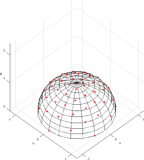
The dome with lights.
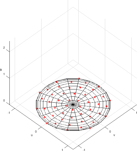
The positions of the lights projected onto the object plane.
Then an exposure is taken from each light in turn yielding \(N\) images and thus \(N\) samples for every pixel position in the images.
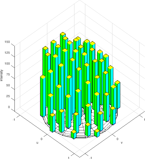
The intensity of one pixel when illuminated by the different lights.
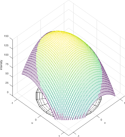
Then a curve is sought that best fits the observed intensities:
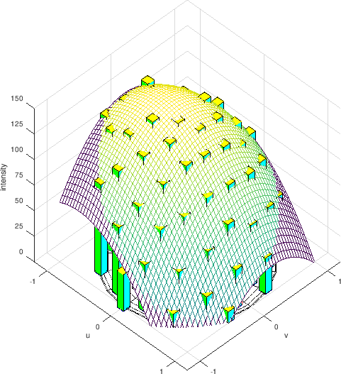
A curve that best fits the observed intensities.
The observed intensities are not needed any more because all we store in the PTM file are the coefficients for the curve.
The curve that is stored in the file. A different one for each pixel.
Because we store 6 coefficients for each pixel in the PTM file (instead of one value in a JPEG file), a PTM file is about 6 times the size of a corresponding JPEG file.
The Math
The polynomial used for curve fitting is:
where \((u,v,w)^T\) is the normalized light vector and \(b\) is the sampled surface luminance. [Malzbender2001]
To fit the curve to the samples we use a Least Squares approximation and solve it using Singular Value Decomposition (SVD). “In the case of an overdetermined system, SVD produces a solution that is the best approximation in the least-squares sense.” [Press2007], Chapter 15.4.2.
Our design matrix:
The vector of samples:
The sought least-squares solution vector:
For each pixel we have to solve:
We do a SVD of \(\mathbf{A}^{N\times6}\) (See [Golub2013], Chapter 2.4):
where \(\sigma_1\geq\sigma_2\geq\dots\geq\sigma_6\geq0.\)
\(\mathbf{U}^{N\times N}\) and \(\mathbf{V}^{6\times6}\) are orthogonal, so their inverses are equal to their transposes, and we can rearrange:
We replace into (2):
\(\boldsymbol{\Sigma}\) is diagonal, so its inverse is the diagonal matrix whose elements are the reciprocals of the elements \(\sigma_1,\dots,\sigma_6\) and we can rearrange for the final least-squares solution of (2):
See: [Press2007], Chapter 2.6.4.
A naive GNU Octave implementation of the PTM is:
function X = ptm(A,b)

[U S V] = svd(A,0)   % 0 requests thin SVD
M       = V * diag (1 ./ diag (S)) * U'
X       = M * b

end
Note that the SVD needs to be computed only once for every different arrangement of light sources. The only part of the above formula that varies for each pixel is \(\mathbf{b}\).
- Drew2009
Drew, M.S. [et al.] 2009, Specularity and Shadow Interpolation via Robust Polynomial Texture Maps https://www.cs.sfu.ca/~mark/ftp/Bmvc09/bmvc09.pdf
- Drew2012
Drew, M.S. [et al.] 2012, Robust Estimation of Surface Properties and Interpolation of Shadow/Specularity Components http://www.cs.sfu.ca/~mark/ftp/Ivc2012/ivc2012.pdf
- Golub2013
Golub, G.H., and Van Loan, C.F. 2013, Matrix Computations, 4th edition, (John Hopkins University Press, Baltimore)
- Lyon2004
A Java implementation of the PTM viewer. https://github.com/clifflyon/ptmviewer
- Malzbender2001(1,2)
Malzbender, T., Gelb, D., and Wolters, H. 2001, Polynomial Texture Maps, http://www.hpl.hp.com/research/ptm/papers/ptm.pdf
- Malzbender2001a
Malzbender, T., and Gelb, D. 2001, Polynomial Texture Map (.ptm) File Format, Version 1.2, http://www.hpl.hp.com/research/ptm/downloads/PtmFormat12.pdf
- Motta2001
Motta, G., Winberger, M.J. 2001, Compression of Polynomial Texture Maps, (HP Laboratories, Palo Alto) http://www.hpl.hp.com/techreports/2000/HPL-2000-143R2.pdf
- Press2007(1,2)
Press, W.H. [et al.] 2007, Numerical recipes: the art of scientifical computing, 3rd edition, (Cambridge University Press, Cambridge)
- Wikipedia
- Zhang2012
Zhang, M., and Drew, M.S. 2012, Robust Luminance and Chromaticity for Matte Regression in Polynomial Texture Mapping in Fusiello, A. [et al.] (Eds.): ECCV 2012 Ws/Demos, Part II, LNCS 7584, pp. 360–369, 2012. Springer, 2012 http://www.cs.sfu.ca/people/Faculty/Drew/ftp/Cpcv2012/cpcv2012a.pdf
- Zhang2014
Zhang, M., and Drew, M.S. 2014, Efficient robust image interpolation and surface properties using polynomial texture mapping, (EURASIP Journal on Image and Video Processing) https://doi.org/10.1186/1687-5281-2014-25